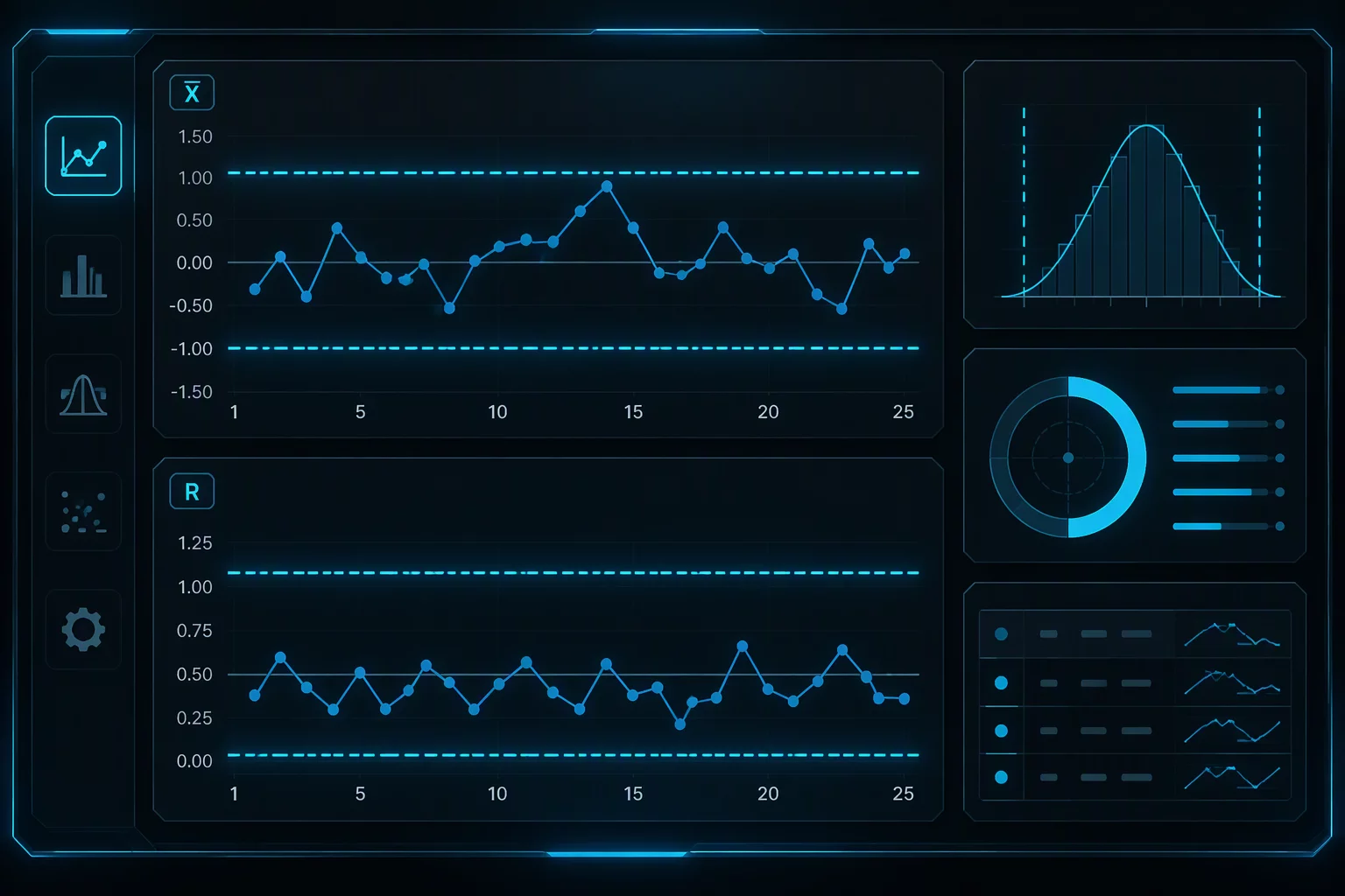
Modeling stochastic variance, running Monte Carlo iterations, and testing parameter sensitivity before committing changes to physical production lines.
Date: August 10, 2026•Author: Tech Editorial•Read Time: 8 min read
Specification Summary
Simulation Architecture & Boundary Parameters
Primary Modeling Engine
Discrete-event and stochastic Monte Carlo simulation runs with empirical distribution mapping
Target Analysis Window
Steady-state operations spanning 2,000 to 50,000 synthetic production cycles
Variance Sensitivity Metric
Non-linear parameter deviation tracking across multi-stage machine tolerances
Verification Standard
Goodness-of-fit cross-validation using historical production baseline logs
Why Simulation Analysis Precedes Physical Line Adjustments
Industrial manufacturing systems rarely behave as deterministic equations on a spreadsheet. Real machinery faces random thermal fluctuations, shifting tool wear, operator cycle variations, and raw material lot inconsistencies. Evaluating process changes directly on physical equipment risks costly line disruptions, out-of-specification scrap, and unrepeatable results. Process simulation analysis creates a mathematically rigorous synthetic twin of the manufacturing environment, allowing engineers to inject stochastic noise and evaluate how upstream variation cascades downstream.
By configuring calibrated input distributions instead of single average values, simulation models reveal latent bottlenecks and unexpected tolerance stack-ups. In high-speed packaging, automated assembly, and continuous chemical processing, this digital sandbox clarifies whether an observed shift in output stems from machine wear or minor feed oscillations. The methodology isolates special-cause signals before any mechanical tool adjustment or recipe modification takes place on the floor.
Consultation Protocol
Request a Simulation Model Review
Submit your production line parameters to receive a structured feasibility review on variance limits and virtual run calibration.
Core Summary
Critical Simulation Benchmarks
Virtual runs must reflect empirical, fitted distributions rather than idealized normal bell curves to avoid masking tail-risk failures.
Upstream cycle time jitter accumulates non-linearly across linked conveyor cells, making buffer sizing crucial.
Sensitivity analysis determines which machine input parameters drive 80 percent of final product dimension drift.
Validation requires comparing synthetic variance spreads against historical baseline control charts before approving line changes.
A single static average conceals the real operational risks; true process simulation measures the shape, spread, and rare extremes of system variability.
— Engineering Systems Group, Technical Fieldbook Notes
System Execution
Virtual Line Calibration & Sensitivity Exploration
Building an effective simulation begins with accurate operational telemetry. Rather than inputting nominal machine speeds, analytical teams record cycle times and physical output measures across varied shifts. These observations are fitted into statistical distributions—such as Weibull for failure intervals or Log-Normal for manual handling durations. Establishing these underlying profiles prevents the simulation from producing overly optimistic throughput estimates.
Once the distribution engine is calibrated, the virtual workflow executes thousands of iterations under controlled variance scenarios. Engineers systematically test stress factors, including batch changeover delays, temperature surges, and feed material irregularities. The following systematic workflow ensures each simulation run delivers actionable engineering intelligence:
Simulation Calibration Sequence
Empirical Baseline Profiling: Capture minimum 500 observational points per machine station to fit authentic probability density functions.
Node Connectivity & Constraint Mapping: Define buffer capacities, conveyor transfer speeds, and routing logic between sequential work cells.
Stochastic Perturbation Runs: Execute 10,000 simulated shifts with randomized variance vectors to expose intermittent blockage points.
Baseline Statistical Alignment: Compare synthetic output distributions with plant SPC charts to verify variance correlation.
Analytical Evaluation
Verification Criteria & Boundary Risk Assessment
A simulation model is only as dependable as its mathematical boundary conditions. If an engineer sets arbitrary lower and upper limits, the model may understate severe deviation events. Cross-referencing model outputs against Anderson-Darling normality assessments and empirical quantile spreads ensures that the simulated variance accurately mirrors real physical behavior under peak load conditions.
When virtual simulation variance matches physical pilot runs within a five percent margin of error, engineers can confidently evaluate hypothetical process adjustments. Operating windows can be widened or narrowed virtually, testing the exact tolerances of new tooling without spending production hours or generating scrap parts. This structured discipline transforms process optimization into a repeatable, risk-controlled science.
Related Material
Complementary Analytical Tool Guides
Control Charts
Real Time SPC Updates and Multilingual Interface Guide
Learn how real-time control chart streaming and localized interfaces improve team responsiveness to manufacturing deviations.