The Average Barely Changed but the Process Became Less Consistent

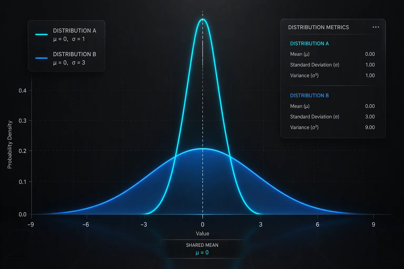
When Centering Hides Deteriorating Uniformity

Production teams frequently celebrate a stable process mean as proof of ongoing health. During an autumn production evaluation on a precision extrusion line, the recorded average wall thickness remained at 4.02 mm across six weeks, almost identical to the nominal specification of 4.00 mm. However, downstream assembly stations abruptly reported sporadic fitment interference.

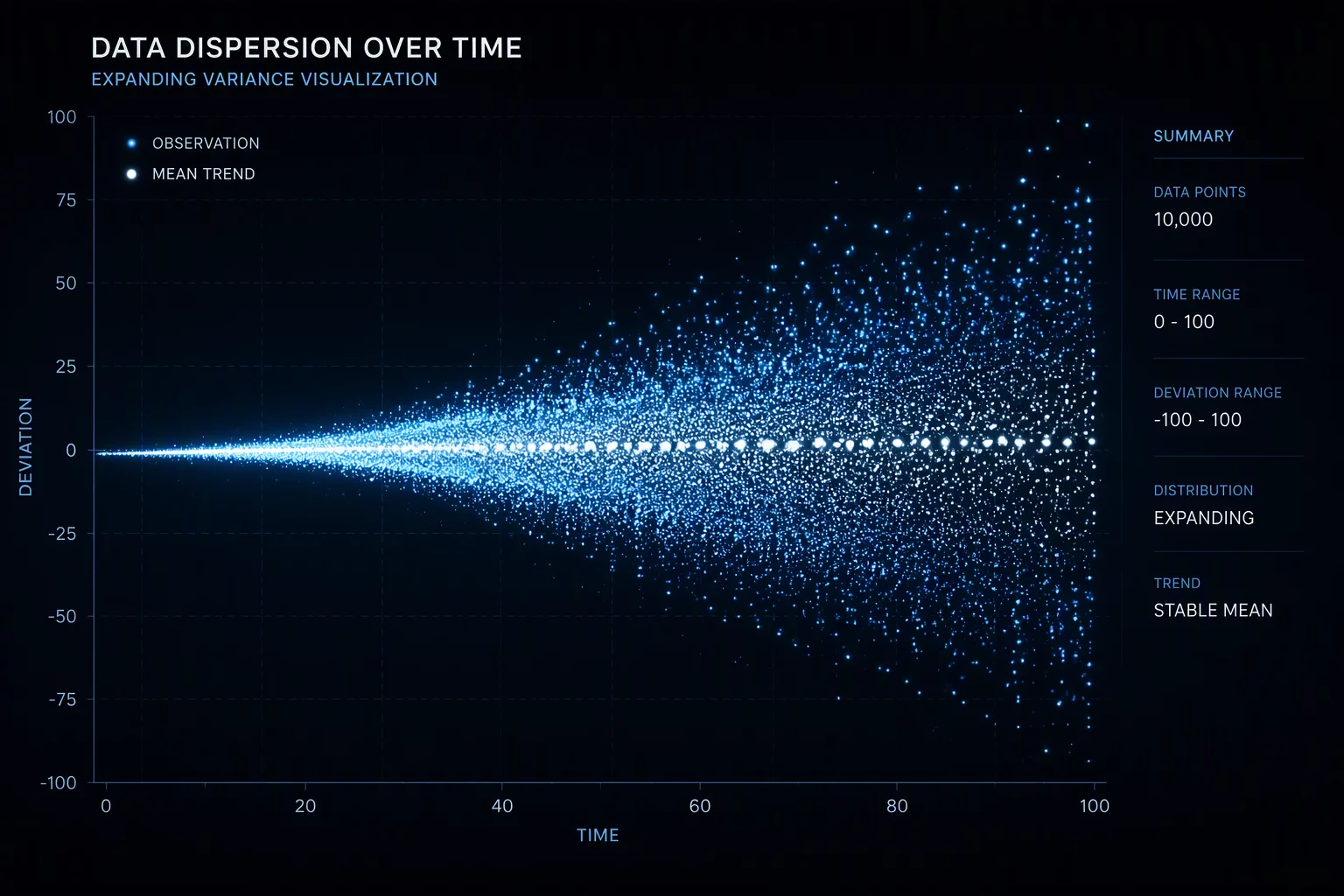
Inspection records revealed that while parts remained within technical tolerances on average, individual piece-to-piece consistency had quietly disintegrated. The operators routinely tracked only average daily outputs, missing the critical widening of the standard deviation from 0.04 mm to 0.082 mm.

• Central tendency monitoring alone provided false operational confidence across both shifts.
• Tooling thermal cycling introduced erratic expansion without pulling the aggregate median.
• Subgroup range values began breaching upper control limits three weeks prior to first customer alerts.

By evaluating moving range and sample standard deviation alongside the arithmetic mean, technicians can promptly decouple centering stability from consistency drift. A process that produces identical averages can nonetheless double its scrap rate if tail tails drift into upper and lower specification limits.

Isolating the True Drivers of Dispersion

Statistical investigation quickly isolated the root cause: an auxiliary cooling manifold valve was intermittently sticking open during second-shift switchovers. The mechanical issue did not bias the extrusion stream hotter or colder overall, but rather alternated rapid chilled cycles with lingering heat. The resulting mixture of fast-cooled and slow-cooled parts canceled out mathematically in sample averages while doubling subgroup dispersion.

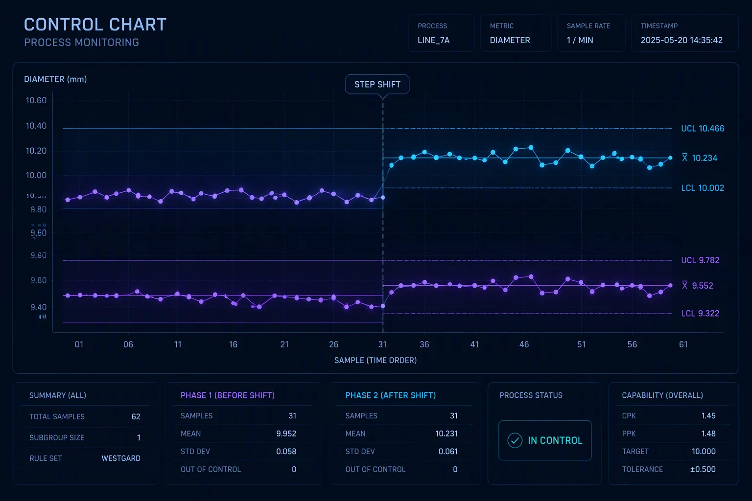
When plotted on an X-bar and S chart, the X-bar chart presented an exemplary run with all points hovering tightly within one standard deviation of the centerline. In contrast, the S chart displayed repeated non-random upward runs and eight consecutive points above the centerline. The disparity demonstrated why dual-chart monitoring is an indispensable prerequisite before accepting any baseline stability hypothesis.

Upgrading Charting Protocols and Sampling Windows

Remediating quiet variance inflation requires tightening the link between dispersion charts and operator reaction plans. The engineering group restructured standard operating procedures: out-of-control rules on S charts now trigger immediate manifold pressure inspections, preventing maintenance delays caused by looking solely for mean drift.

Furthermore, rational subgrouping was redefined to capture consecutive parts within distinct machine cycles rather than pooling pieces across shift handoffs. This prevented internal variation within batches from masquerading as acceptable common-cause noise, establishing true baseline visibility across all operating envelopes.