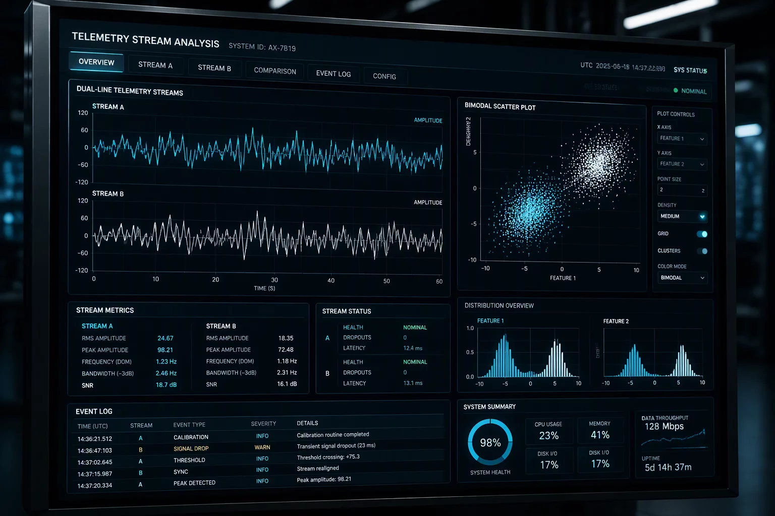
How Dual Operating Conditions Contaminate Reference Windows
Process baselines establish the expected voice of an operation, serving as the benchmark against which future stability and process capability are judged. In this production review, engineering teams recorded 420 consecutive hourly runs into a single control chart baseline, assuming homogeneous continuous processing.
Subsequent runs routinely triggered false alarms during low-throughput cycles while completely failing to flag significant variance during peak operational cycles. The historical log revealed an unrecorded reality: the line operated at 1,200 units per hour during morning shifts and throttled back to 850 units per hour during late shifts due to upstream thermal cooling limits.
- Aggregating disparate operating temperatures and feed rates directly created a bimodal distribution disguised as standard common cause variation.
- Standard deviation calculated across both regimes inflated the three-sigma control limits by approximately 38 percent.
- True process changes during standard operations remained invisible because broad control limits accepted unstable outliers.
A baseline must reflect a single, coherent operating condition. When multiple physical states get collapsed into one sample population, the mathematical foundation of statistical process control breaks down, turning control charts into deceptive administrative dashboards.
“A control chart cannot distinguish between special causes and common variation if the baseline itself is built on two conflicting physical regimes.”
Deconstructing the Bimodal Baseline and Control Limits
When evaluating historical run charts, normal distribution tests often flag skewness or excessive kurtosis that engineers mistakenly attribute to measurement noise. In this assembly case, a stratified histogram immediately separated into two distinct Gaussian peaks centered around separate local averages. The high-speed regime operated with an average cycle time of 48.2 seconds, while the throttled regime settled near 54.6 seconds.
Calculating a single grand average of 51.4 seconds produced an artificial center line where almost no actual parts were manufactured. Points oscillated back and forth across the center line, creating artificial stratification and suppressing natural run rules. Rather than signaling a stable process, the narrow distance between points and the center line was an artifact of inflated dispersion formulas calculated from mixed variances.
Stratification, Window Segmentation, and Phase Management
Resolving contaminated baselines requires strict parameter partitioning rather than post-hoc mathematical filtering. Engineering teams isolated the 420 batch logs by feed rate and thermal setpoints, calculating separate three-sigma limits for each confirmed operational state. Once partitioned into discrete baseline windows, each operating mode exhibited predictable common cause variation with tightly bounded limits.
Future process reviews now mandate recording operating parameters alongside quality metrics before compiling baseline datasets. Dynamic control chart phasing allows real-time dashboards to toggle between regime-specific limits automatically, restoring statistical sensitivity and eliminating both phantom alarms and undetected operational shifts.
Related Articles

Frequently Asked Questions
When two distinct operating conditions are grouped together, the difference between their individual averages is treated as inherent random error. This inflated variability expands the distance between upper and lower control limits, severely desensitizing the chart.
It can only share a chart if data points are standardized against each regime's specific mean and standard deviation (z-score transformations), or if the chart uses distinct phases with stepped control limits for each operational mode.
Test the baseline distribution for multimodality using histograms or probability plots, cross-reference data clusters with time-of-day or machine logs, and evaluate whether points clump closely around the overall average without approaching the limits.
Key Analytical Takeaways
Baselines must represent a singular physical operating condition to avoid conflating deliberate machine setpoints with common cause variation.
Mixed operating windows inflate the standard deviation, spreading control limits too wide and masking genuine special-cause signals.
Partition historical datasets into distinct phases or utilize normalized deviation charts whenever operating conditions change by design.
Request Analytical Consultation
Inquire directly on statistical baseline validation and review specific parameters of this case.